VarDecomp can be used for variance decomposition, model fit checks and output visualizations of brms models.
Installation
You can install the development version of VarDecomp like so:
devtools::install_github("gabewinter/VarDecomp")Documentation
Full documentation website on: https://gabewinter.github.io/VarDecomp
Example
library(tidyverse)
md = tibble(
sex = sample(rep(c(-0.5, 0.5), each = 500)),
species = sample(rep(c("species1","species2","species3","species4","species5"), each = 200))) %>%
## Create a variables
dplyr::mutate(height = rnorm(1000, mean = 170, sd = 10),
mass = 5 + 0.5 * height + rnorm(1000, mean = 0, sd = 5)) %>%
dplyr::mutate(height = height - mean(height),
mass = log(mass))
mod = brms_model(Chainset = 2,
Response = "mass",
FixedEffect = c("sex","height"),
Family = "gaussian",
Data = md)
#> [1] "No problems so far 🙌"
#> Compiling Stan program...
#> Start sampling
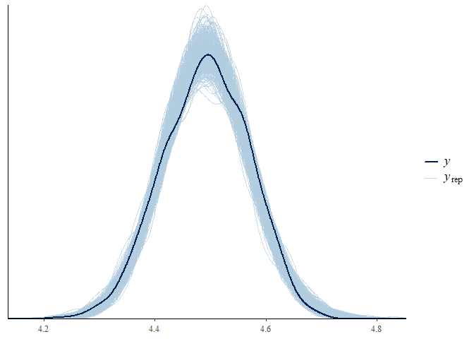
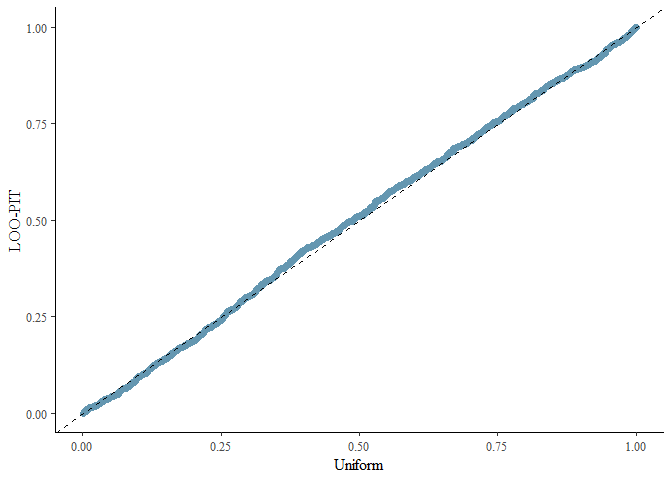
model_fit(mod, Group = "sex")
#> No divergences to plot.
#> Using all posterior draws for ppc type 'loo_pit_qq' by default.
#> Using all posterior draws for ppc type 'violin_grouped' by default.
#> $`R-hat and Effective sample size`
#> # A tibble: 1 × 2
#> Rhat EffectiveSampleSize
#> <dbl> <dbl>
#> 1 1.00 1650.
#>
#> $`Traceplots plot`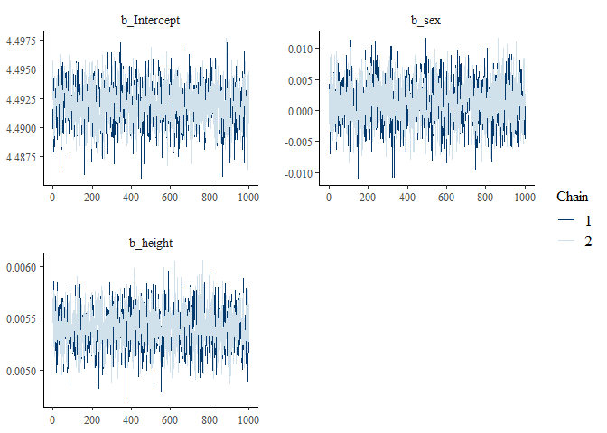
#>
#> $`Posterior predictive check - Group density overlay plot`
#> $`Posterior predictive check - Group density overlay plot`$GroupPlot_sex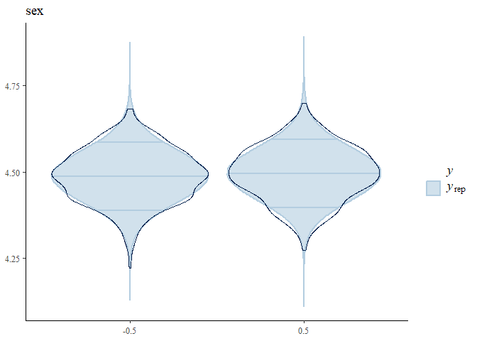
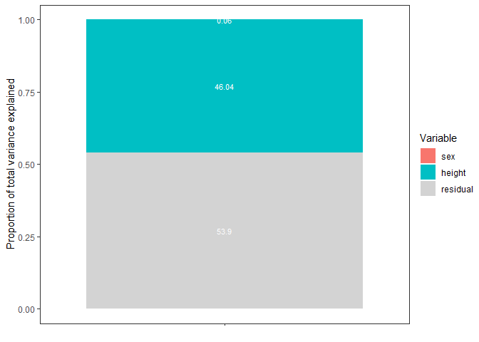
model_summary(mod)
#> # A tibble: 7 × 6
#>   variable              mean median    sd lower_HPD upper_HPD
#>   <chr>                <dbl>  <dbl> <dbl>     <dbl>     <dbl>
#> 1 Intercept            4.49   4.49  0.002     4.49      4.50
#> 2 sex                  0.001  0.001 0.004    -0.006     0.008
#> 3 height               0.005  0.005 0         0.005     0.006
#> 4 R2_sex               0.001  0     0.001     0         0.002
#> 5 R2_height            0.46   0.461 0.021     0.417     0.499
#> 6 R2_sum_fixed_effects 0.461  0.462 0.021     0.418     0.499
#> 7 R2_residual          0.539  0.538 0.021     0.501     0.582

plot_intervals(mod)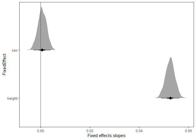
PS = var_decomp(mod)

plot_R2(PS)