Perform model fit checks for brms models

model_fit(brmsfit, Prior = FALSE)

Arguments

brmsfit: The output of a brms model. You can use VarDecomp::brms_model() to produce a brmsfit.
Prior: A logical argument defining whether the brmsfit contains prior samples. If set to TRUE it will produce plots comparing the log distributions of priors and posterior samples for each covariate.

Value

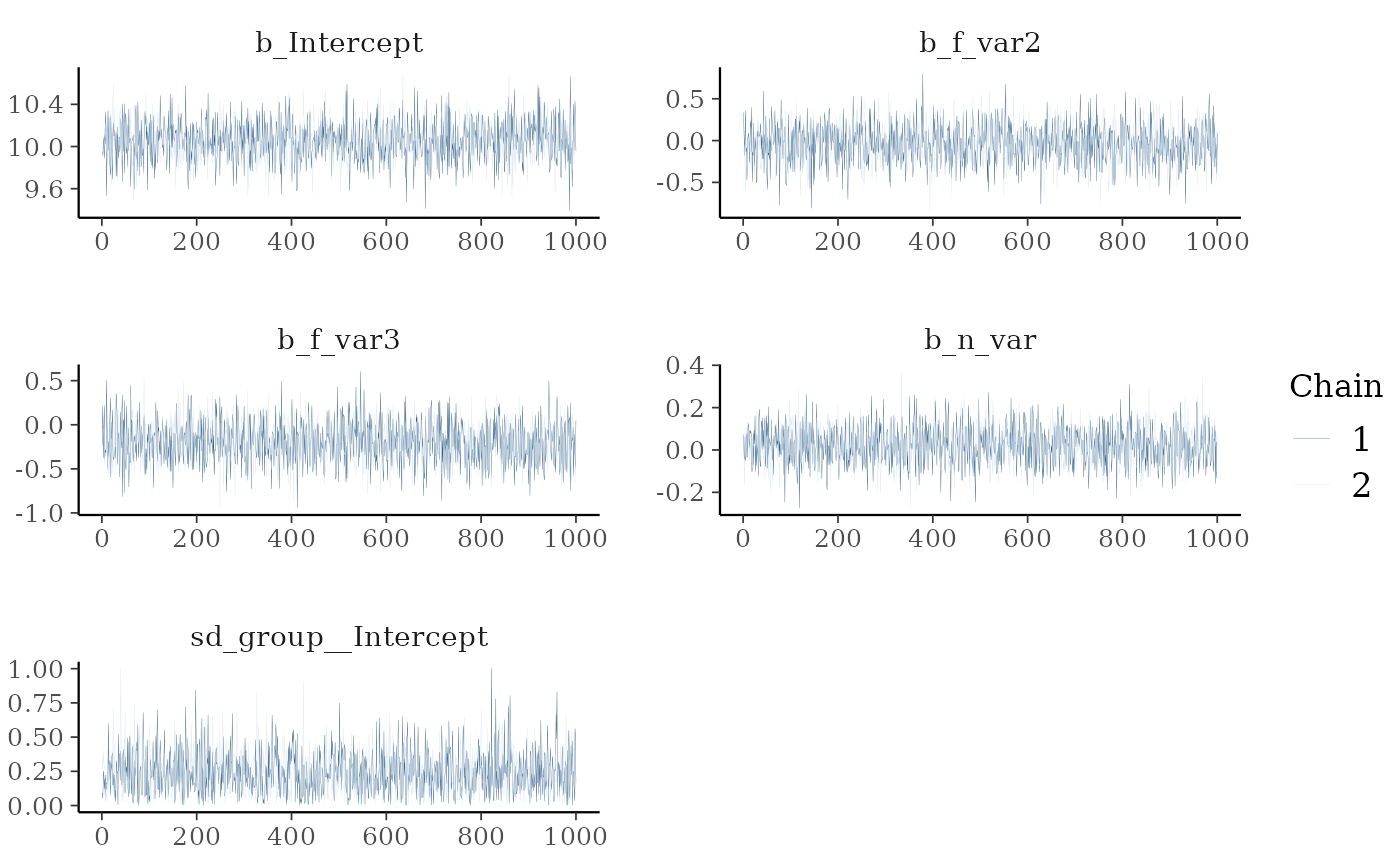
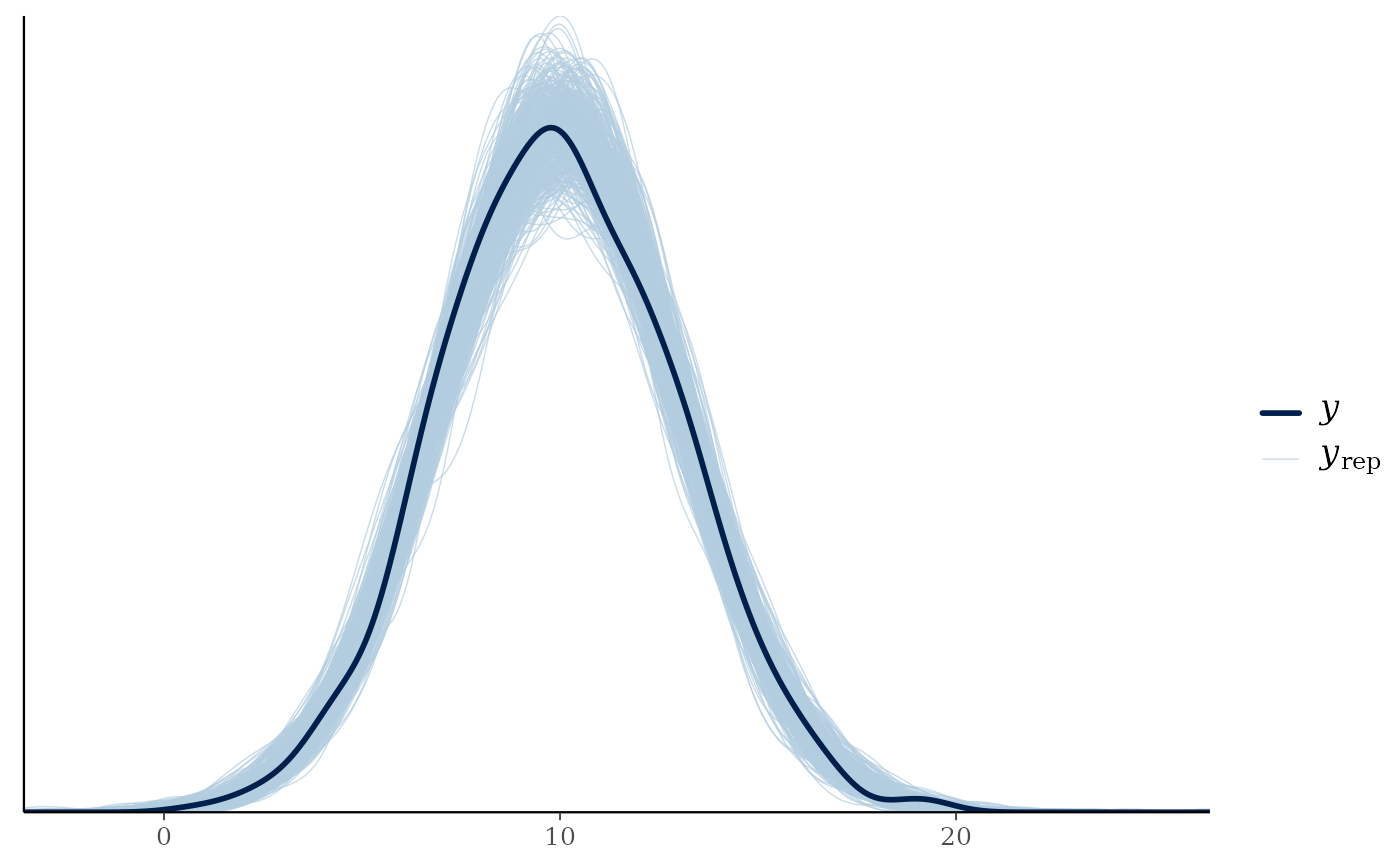
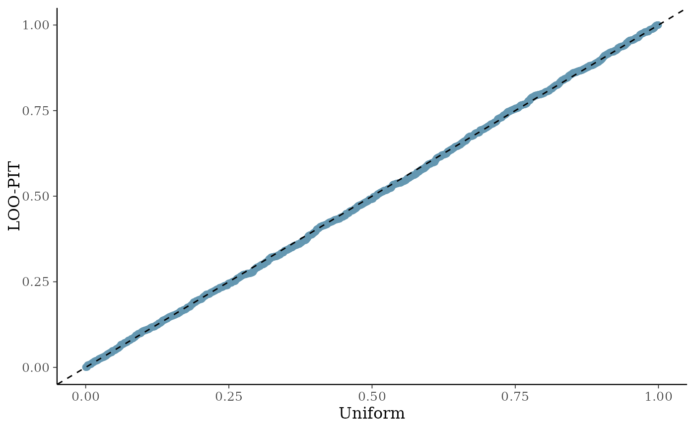
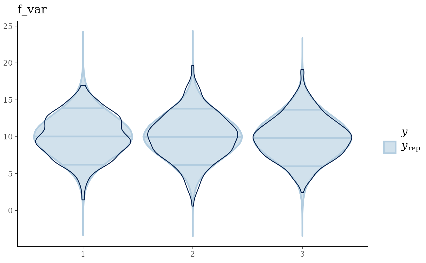
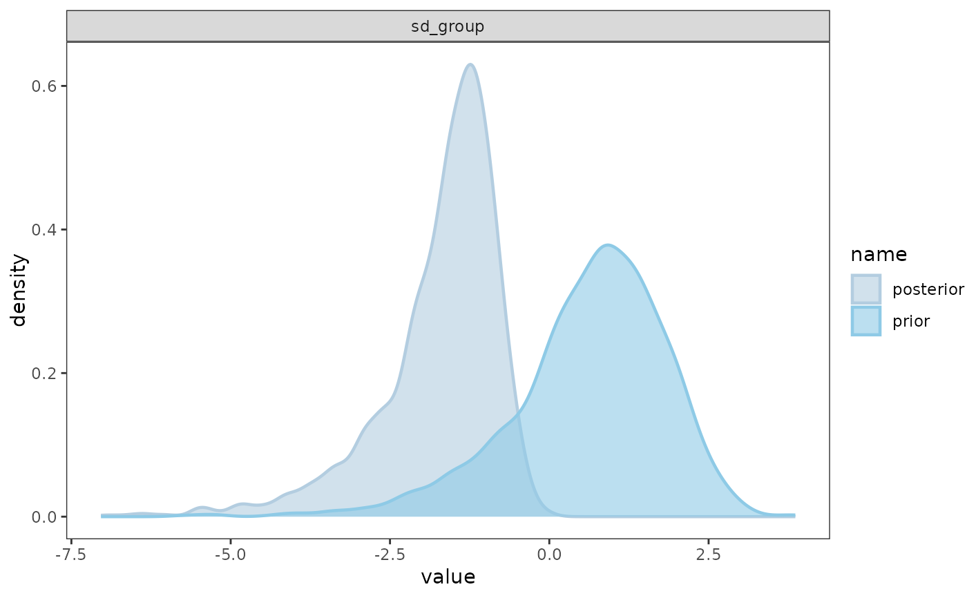
Returns a list containing (a) the maximum R-hat value, (b) the minimum effective sample size, (c) traceplots, (d) posterior predictive check plots, and (e) prior and posterior sample plots (if priors are available).

Examples


# Simulate data
md = tibble::tibble(
  group = factor(sample(1:10, 1000, replace = TRUE)),
  f_var = factor(sample(1:3, 1000, replace = TRUE)),
  n_var = rnorm(1000, mean = 0, sd = 1),
  resp = rnorm(1000, mean = 10, sd = 3))

# Run model
mod = brms_model(Response = "resp", 
                 FixedEffect = c("f_var","n_var"), 
                 RandomEffect = "group", 
                 Family = "gaussian", 
                 Data = md)
#> [1] "No problems so far 🙌"
#> Compiling Stan program...
#> Start sampling


# Check model fit 
model_fit(mod, Prior = TRUE)
#> No divergences to plot.
#> Using all posterior draws for ppc type 'violin_grouped' by default.
#>       Rhat EffectiveSampleSize
#> 1 1.001913            1657.166
#> n 2: Gradient evaluation took 0.000207 seconds
#> Chain 2: 1000 transitions using 10 leapfrog steps per transition would take 2.07 seconds.
#> Chain 2: Adjust your expectations accordingly!
#> Chain 2: 
#> Chain 2: 
#> Chain 1: Iteration:     1 / 30000 [  0%]  (Warmup)
#> Chain 2: Iteration:     1 / 30000 [  0%]  (Warmup)
#> Chain 1: Iteration:  3000 / 30000 [ 10%]  (Warmup)
#> Chain 2: Iteration:  3000 / 30000 [ 10%]  (Warmup)
#> Chain 1: Iteration:  6000 / 30000 [ 20%]  (Warmup)
#> Chain 2: Iteration:  6000 / 30000 [ 20%]  (Warmup)
#> Chain 1: Iteration:  9000 / 30000 [ 30%]  (Warmup)
#> Chain 2: Iteration:  9000 / 30000 [ 30%]  (Warmup)
#> Chain 2: Iteration: 12000 / 30000 [ 40%]  (Warmup)
#> Chain 1: Iteration: 12000 / 30000 [ 40%]  (Warmup)
#> Chain 2: Iteration: 15000 / 30000 [ 50%]  (Warmup)
#> Chain 2: Iteration: 15001 / 30000 [ 50%]  (Sampling)
#> Chain 1: Iteration: 15000 / 30000 [ 50%]  (Warmup)
#> Chain 1: Iteration: 15001 / 30000 [ 50%]  (Sampling)
#> Chain 2: Iteration: 18000 / 30000 [ 60%]  (Sampling)
#> Chain 1: Iteration: 18000 / 30000 [ 60%]  (Sampling)
#> Chain 2: Iteration: 21000 / 30000 [ 70%]  (Sampling)
#> Chain 1: Iteration: 21000 / 30000 [ 70%]  (Sampling)
#> Chain 2: Iteration: 24000 / 30000 [ 80%]  (Sampling)
#> Chain 1: Iteration: 24000 / 30000 [ 80%]  (Sampling)
#> Chain 2: Iteration: 27000 / 30000 [ 90%]  (Sampling)
#> Chain 1: Iteration: 27000 / 30000 [ 90%]  (Sampling)
#> Chain 2: Iteration: 30000 / 30000 [100%]  (Sampling)
#> Chain 2: 
#> Chain 2:  Elapsed Time: 58.138 seconds (Warm-up)
#> Chain 2:                59.767 seconds (Sampling)
#> Chain 2:                117.905 seconds (Total)
#> Chain 2: 
#> Chain 1: Iteration: 30000 / 30000 [100%]  (Sampling)
#> Chain 1: 
#> Chain 1:  Elapsed Time: 58.862 seconds (Warm-up)
#> Chain 1:                65.561 seconds (Sampling)
#> Chain 1:                124.423 seconds (Total)
#> Chain 1: